
RNA-Seq data Analysis
RNA-seq experiments are performed with an aim to comprehend transcriptomic changes in organisms in response to a certain treatment. They are also designed to understand the cause and/or effect of a mutation by measuring the resulting gene expression changes. Thanks to some robust algorithms specifically designed to map short stretches of nucleotide sequences to a genome while being aware of the process of RNA splicing has led to many advances in RNAseq analysis. The overview of RNA-seq analysis is summarized in Fig1.
Overview

This document will guide you through basic RNAseq analysis, beginning at quality checking of the RNAseq reads through to getting the differential gene expression results. We have downloaded an Arabidopsis dataset from NCBI for this purpose. Check the BioProject ⤴ page for more information.
Experimental design
This experiment compares WT and atrx-1 mutant to analyze how the loss of function of ATRX chaperone results in changes in gene expression. The ATRX chaperone is a histone chaperone known to be an important player in the regulation of gene expression. RNA was isolated from three WT replicates and three mutant replicates using Trizol. The transcriptome was enriched/isolated using the plant RiboMinus kit for obtaining total RNA. RNA-seq was carried out in Illumina Hiseq 2500. The sequencing reads were generated as paired-end data, hence we have 2 files per replicate.
| Condition | replicate 1 | replicate 2 | replicate 3 |
|---|---|---|---|
| WT | SRR4420293_1.fastq.gz SRR4420293_2.fastq.gz |
SRR4420294_1.fastq.gz SRR4420294_2.fastq.gz |
SRR4420295_1.fastq.gz SRR4420295_2.fastq.gz |
| atrx-1 | SRR4420296_1.fastq.gz SRR4420296_2.fastq.gz |
SRR4420297_1.fastq.gz SRR4420297_2.fastq.gz |
SRR4420298_1.fastq.gz SRR4420298_2.fastq.gz |
Raw Sequence Data
Generally, if the data is hosted at your local sequencing center, you could download it through a web interface or using wget or curl commands. However in this example, we will download data hosted on public repositories. There are several public data repositories that host the data.
1. Download the data from public repositories
A) EMBL-EBI’s European Nucletide Archive (ENA)
The best option is to download the fastq files directly from the ENA server (e.g., check EBI ⤴). We can download them directly using wget by supplying the download links to each file; for example, in this case:
1
2
3
4
5
6
7
8
9
10
11
12
13
wget ftp://ftp.sra.ebi.ac.uk/vol1/fastq/SRR442/003/SRR4420293/SRR4420293_1.fastq.gz
wget ftp://ftp.sra.ebi.ac.uk/vol1/fastq/SRR442/003/SRR4420293/SRR4420293_2.fastq.gz
wget ftp://ftp.sra.ebi.ac.uk/vol1/fastq/SRR442/004/SRR4420294/SRR4420294_1.fastq.gz
wget ftp://ftp.sra.ebi.ac.uk/vol1/fastq/SRR442/004/SRR4420294/SRR4420294_2.fastq.gz
wget ftp://ftp.sra.ebi.ac.uk/vol1/fastq/SRR442/005/SRR4420295/SRR4420295_1.fastq.gz
wget ftp://ftp.sra.ebi.ac.uk/vol1/fastq/SRR442/005/SRR4420295/SRR4420295_2.fastq.gz
wget ftp://ftp.sra.ebi.ac.uk/vol1/fastq/SRR442/006/SRR4420296/SRR4420296_1.fastq.gz
wget ftp://ftp.sra.ebi.ac.uk/vol1/fastq/SRR442/006/SRR4420296/SRR4420296_2.fastq.gz
wget ftp://ftp.sra.ebi.ac.uk/vol1/fastq/SRR442/007/SRR4420297/SRR4420297_1.fastq.gz
wget ftp://ftp.sra.ebi.ac.uk/vol1/fastq/SRR442/007/SRR4420297/SRR4420297_2.fastq.gz
wget ftp://ftp.sra.ebi.ac.uk/vol1/fastq/SRR442/008/SRR4420298/SRR4420298_1.fastq.gz
wget ftp://ftp.sra.ebi.ac.uk/vol1/fastq/SRR442/008/SRR4420298/SRR4420298_2.fastq.gz
B) National Center for Biotechnology Information (NCBI)
The data is hosted as SRA (Sequence Read Archives) files on the public archives in NCBI. We can bulk download these using aspera high-speed file transfer.
It is common to install software as environmental modules on your compute cluster. So we begin by loading the relevant modules. The following code expects that you have sra-toolkit, GNU parallel, and aspera installed on your computing cluster.
Sometimes, a user might run into perl issues while using edirect. The installed version of perl should support the HTTPS protocol.
Run the code snippet in the terminal window:
1
2
3
4
5
6
7
8
9
10
11
12
module load <path/to/sra-toolkit>
module load <path/to/edirect>
module load <path/to/parallel>

esearch -db sra -query PRJNA348194 | \
  efetch --format runinfo |\
  cut -d "," -f 1 | \
  awk 'NF>0' | \
  grep -v "Run" > srr_numbers.txt

while read line; do echo "prefetch --max-size 100G --transport ascp --ascp-path \"/path/to/aspera/.../ascp|/path.../etc/asperaweb_id_dsa.openssh\" ${line}"; done < srr_numbers.txt > prefetch.cmds
parallel < prefetch.cmds
After downloading the SRA files, we convert them to fastq format. We can use the fast-dump command as follows: (this step is slow, so if possible, run these commands using GNU parallel ⤴). We assume that all SRA files are in a specific folder.
1
2
3
module load parallel
INDIR=/path/to/sra/files/        # Folder containing input SRA files for fastq-dump
parallel fastq-dump --split-files --origfmt --gzip" ::: ${INDIR}/*.sra
Note that
fastq-dump runs very slow.
We also need the genome file and associated GTF/GFF file for Arabidopsis. These are downloaded directly from NCBI ⤴, or plants Ensembl website ⤴, or the Phytozome website ⤴. (^The Phytozome needs logging in and selecting the files.)
For this tutorial, we downloaded the following files from NCBI ⤴:
1
2
3
Genome Fasta File: GCF_000001735.3_TAIR10_genomic.fna
Annotation file: GCF_000001735.3_TAIR10_genomic.gff
We can use wget to fetch both the Genome (Fasta) file and the Annotation (GFF) file:
1
2
wget https://ftp.ncbi.nlm.nih.gov/genomes/all/GCF/000/001/735/GCF_000001735.4_TAIR10.1/GCF_000001735.4_TAIR10.1_genomic.fna.gz
wget https://ftp.ncbi.nlm.nih.gov/genomes/all/GCF/000/001/735/GCF_000001735.4_TAIR10.1/GCF_000001735.4_TAIR10.1_genomic.gff.gz
2. Quality Check
We use fastqc, a tool that provides a simple way to do quality control checks on raw sequence data coming from high throughput sequencing pipelines (FastQC ⤴).
Watch the video below to check the quality of high throughput sequence using FastQC [source: BabrahamBioinf ⤴ ]
It uses various metrics to indicate how your data is. A high-quality Illumina RNAseq file should look something like this ⤴. Since there are 6 sets of files (12 files total), we need to run fastqc on each one of them. It is convenient to run it in parallel.
1
2
3
4
5
6
7
module load fastqc
module load parallel

mkdir fq_out_directory
OUTDIR=fq_out_directory

parallel "fastqc {} -o ${OUTDIR}" ::: *.fastq.gz
Because we have in total 6 quality outputs, we will have 6 HTML files and 6 zip files. We can use MultiQC ⤴ to aggregate the outputs and get a single HTML file detailing the data quality of all the libraries.
1
2
3
4
5
6
7
8
9
10
11
12
13
14
cd fq_out_directory
module load python/3           # may need to search for multiqc module
module load py-multiqc         # if not found, try 'module avail multiqc'

multiqc .
[INFO   ]         multiqc : This is MultiQC v0.8
[INFO   ]         multiqc : Template    : default
[INFO   ]         multiqc : Searching '.'
[INFO   ]          fastqc : Found 6 reports
[INFO   ]         multiqc : Report      : multiqc_report.html
[INFO   ]         multiqc : Data        : multiqc_data
[INFO   ]         multiqc : MultiQC complete
This will give you a combined HTML file and a folder named multiqc_data with containing three files describing the various statistics:
1
2
3
4
5
6
7
8
9
10
11
ls
multiqc_data (Folder)
multiqc_report.html

cd multiqc_data
ls

multiqc_fastqc.txt
multiqc_general_stats.txt
multiqc_sources.txt
..........
You can peruse the complete report or download the plots and view them, for example:
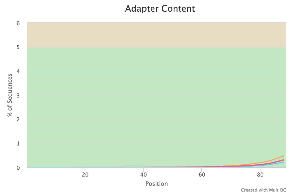
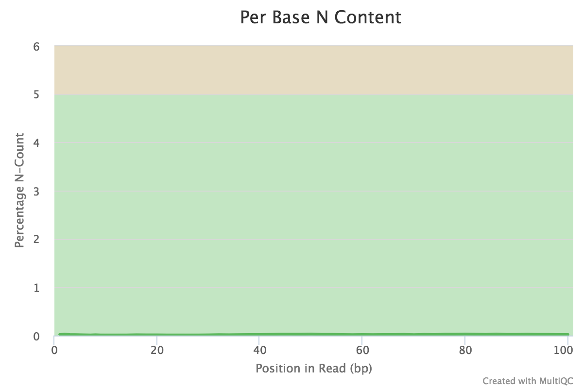
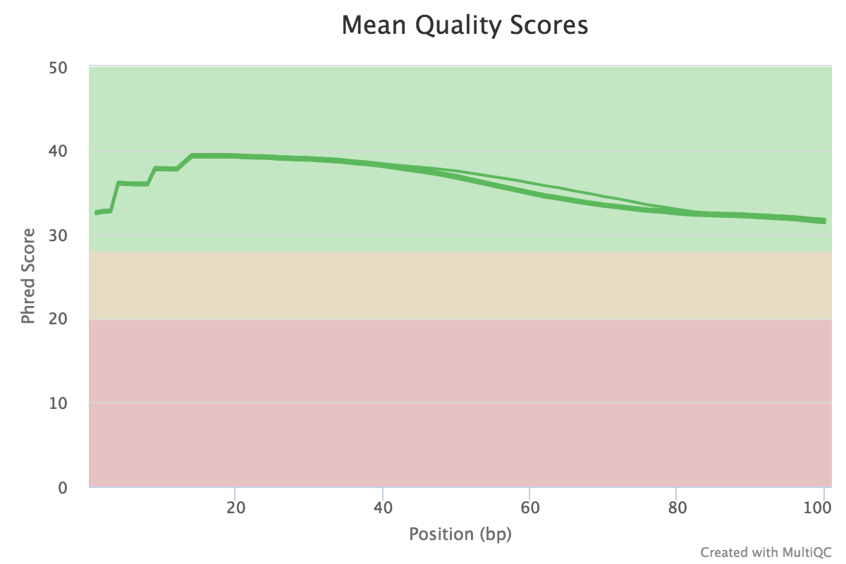
If satisfied with the results, proceed with the mapping. If not, then perform quality trimming. For example, see here ⤴. If the quality is very bad, excluding that sample from the analysis might make more sense.
3. Mapping reads to the genome
There are several mapping programs available for aligning RNAseq reads to the genome. Generic aligners such as BWA, bowtie2, BBMap, etc., are not suitable for mapping RNAseq reads because they are not splice-aware. RNAseq reads are mRNA reads that only contain exonic regions, hence mapping them back to the genome requires splitting the individual reads that span an intron. It can be done only by splice-aware mappers. In this tutorial, we will use HISAT2 ⤴, a successor of Tophat2.
HiSat2 for mapping
Hisat2 indexing
For HiSat2 mapping, you first need to index the genome and then use the read pairs to map the indexed genome (one set at a time). For indexing the genome, we use the hisat2-build command as follows in a SLURM script:
^ Learn more about slurm ⤴ from the hands-on tutorial.
1
2
3
4
5
6
7
8
9
10
11
12
13
14
15
16
17
18
19
20
21
22
23
#!/bin/bash

#SBATCH -N 1
#SBATCH --ntasks-per-node=16
#SBATCH --time=24:00:00
#SBATCH --job-name=HI_build
#SBATCH --output=HI_build.%j.out
#SBATCH --error=HI_build.%j.err
#SBATCH --mail-user=<user_email_address>
#SBATCH --mail-type=begin
#SBATCH --mail-type=end

set -o xtrace
cd ${SLURM_SUBMIT_DIR}
scontrol show job ${SLURM_JOB_ID}
ulimit -s unlimited

module load hisat2

GENOME_FNA="/path/to/refrence/GCF_000001735.3_TAIR10_genomic.fna"
GENOME=${GENOME_FNA%.*}                # Drops the .fna extension
hisat2-build ${GENOME_FNA} ${GENOME}
Let’s go to your working directory, where you downloaded the genome file. Create an empty file using the touch indexing_hisat2.sh command, open it using your favorite text editor in the terminal (e.g., nano or vim) and copy-paste the script from above. Find the GENOME_FNA= variable and update the path and filename of the genomic file. Save changes and submit the script into the SLURM queue:
1
sbatch indexing_hisat2.sh
Note to update the path and filename of the reference genome in the GENOME_FNA variable. If the downloaded file is zipped, decompress it before running the script:
gzip -d {filename}.fna.gz
Adjust the #SBATCH --time variable, provided in format hours:minutes:seconds. The provided value allocates the time at the computational node. If your setup is too short, the task will be interrupted prefinal. Otherwise, if it is too long, you will have a long wait in the queue.
Setting up #SBATCH --time=1:00:00 is sufficient for indexing the genome in this example.
Once complete, you should see several files with the .ht2 extension. These are the index files.
1
2
3
4
5
6
7
8
 GCF_000001735.3_TAIR10_genomic.1.ht2
 GCF_000001735.3_TAIR10_genomic.2.ht2
 GCF_000001735.3_TAIR10_genomic.3.ht2
 GCF_000001735.3_TAIR10_genomic.4.ht2
 GCF_000001735.3_TAIR10_genomic.5.ht2
 GCF_000001735.3_TAIR10_genomic.6.ht2
 GCF_000001735.3_TAIR10_genomic.7.ht2
 GCF_000001735.3_TAIR10_genomic.8.ht2
If outputs were not generated, check the HI_build.{jobID}.err (and HI_build.{jobID}.out) files to detect the reason for the failure.
At the mapping step, we simply refer to the index using GCF_000001735.3_TAIR10_genomic as described in the next step.
Hisat2 Mapping
For mapping, for each set of reads (forward and reverse or R1 and R2), we first set up a run_hisat2.sh script as follows:
1
2
3
4
5
6
7
8
9
10
11
12
13
14
15
16
17
18
19
20
21
22
23
24
25
26
27
28
29
30
31
32
33
#!/bin/bash

set -o xtrace

# set the reference index:
GENOME="/path/to/refrence/GCF_000001735.3_TAIR10_genomic"

# make an output directory to store the output aligned files
OUTDIR="/path/to/out_dir"
[[ -d ${OUTDIR} ]] || mkdir -p ${OUTDIR}        # If output directory doesn't exist, craete it

p=8 # use 8 threads
R1_FQ="$1" # first argument
R2_FQ="$2" # second argument

# purge and load relevant modules.
module purge

module load hisat2
module load samtools

OUTFILE=$(basename ${R1_FQ} | cut -f 1 -d "_");

hisat2 \
  -p ${p} \
  -x ${GENOME} \
  -1 ${R1_FQ} \
  -2 ${R2_FQ} \
  -S ${OUTDIR}/${OUTFILE}.sam &> ${OUTFILE}.log
samtools view --threads ${p} -bS -o ${OUTDIR}/${OUTFILE}.bam ${OUTDIR}/${OUTFILE}.sam

rm ${OUTDIR}/${OUTFILE}.sam
For setup to run with each set of files, we can set a SLURM script (loop_hisat2.sh) that loops over each fastq file. Note that this script calls the run_hisat2.sh script for each pair of fastq files supplied as its argument.
1
2
3
4
5
6
7
8
9
10
11
12
13
14
15
16
17
18
19
20
21
22
#!/bin/bash

#SBATCH -N 1
#SBATCH --ntasks-per-node=16
#SBATCH --time=24:00:00
#SBATCH --job-name=Hisat2
#SBATCH --output=Hisat2.%j.out
#SBATCH --error=Hisat2.%j.err
#SBATCH --mail-user=<user_email_address>
#SBATCH --mail-type=begin
#SBATCH --mail-type=end

set -o xtrace
cd ${SLURM_SUBMIT_DIR}
ulimit -s unlimited
scontrol show job ${SLURM_JOB_ID}

for fq1 in *1.*gz; do
  fq2=$(echo ${fq1} | sed 's/1/2/g');
  bash run_hisat2.sh ${fq1} ${fq2};
done &> hisat2_1.log
Now submit this job as follows:
1
sbatch loop_hisat2.sh
That should create the following files as output:
1
2
3
4
5
6
SRR4420298.bam
SRR4420297.bam
SRR4420296.bam
SRR4420295.bam
SRR4420294.bam
SRR4420293.bam
STAR for mapping
STAR Index
4. Abundance estimation
For quantifying transcript abundance from RNA-seq data, there are many programs available. Two most popular tools include, featureCounts and HTSeq. We will need a file with aligned sequencing reads (SAM/BAM files generated in previous step) and a list of genomic features (from the GFF file). featureCounts is a highly efficient general-purpose read summarization program that counts mapped reads for genomic features such as genes, exons, promoter, gene bodies, genomic bins and chromosomal locations. It also outputs stat info for the overall summarization results, including number of successfully assigned reads and number of reads that failed to be assigned due to various reasons. We can run featureCounts on all SAM/BAM files at the same time or individually.
featureCounts
You will need subread ⤴ and parallel modules loaded.
1
2
3
4
5
6
7
8
9
10
11
12
13
14
15
16
17
18
19
20
21
22
23
24
25
26
27
28
29
#!/bin/bash

#SBATCH -N 1
#SBATCH --ntasks-per-node=16
#SBATCH --time=24:00:00
#SBATCH --job-name=Hisat2
#SBATCH --output=Hisat2.%j.out
#SBATCH --error=Hisat2.%j.err
#SBATCH --mail-user=<user_email_address>
#SBATCH --mail-type=begin
#SBATCH --mail-type=end

set -o xtrace

cd ${SLURM_SUBMIT_DIR}
ulimit -s unlimited
ANNOT_GFF="/PATH/TO/GFF_FILE"          # file should be decompressed, e.g., gzip -d {filename}.gff.gz
INDIR="/Path/TO/BAMFILES/DIR"
OUTDIR=counts
[[ -d ${OUTDIR} ]] || mkdir -p ${OUTDIR}

module purge

module load subread
module load parallel

parallel -j 4 "featureCounts -T 4 -s 2 -p -t gene -g ID -a ${ANNOT_GFF} -o ${OUTDIR}/{/.}.gene.txt {}" ::: ${INDIR}/*.bam
scontrol show job ${SLURM_JOB_ID}
Let’s go to your working directory, where you downloaded and decompressed the annotation (GFF) file. Create an empty file using the touch run_feature_counts.sh command, open it using your favorite text editor in the terminal (e.g., nano or vim) and copy-paste the script from above. Find the ANNOT_GFF= variable and update the path and filename of the annotation file. Also, update the INDIR= variable using path to the directory with BAM files from the previous step. Save changes and submit the script into the SLURM queue:
1
sbatch run_feature_counts.sh
This creates the following set of files in the specified output folder:
Count Files:
1
2
3
4
5
6
SRR4420298.gene.txt
SRR4420293.gene.txt
SRR4420297.gene.txt
SRR4420296.gene.txt
SRR4420295.gene.txt
SRR4420294.gene.txt
Each file has a commented line starting with a # which gives the command used to create the count table and the relevant seven columns as follows, for example:
head SRR4420298.gene.txt
1
2
3
4
5
6
7
8
9
10
11
12
# Program:featureCounts v1.5.2; Command:"featureCounts" "-T" "4" "-s" "2" "-p" "-t" "gene" "-g" "ID" "-a" "/path/to/GCF_000001735.3_TAIR10_genomic.gff" "-o" "/path/to/counts/SRR4420298.gene.txt" "SRR4420298.bam"

Geneid  Chr     Start   End     Strand  Length  SRR4420298.bam
gene0   NC_003070.9     3631    5899    +       2269    13
gene1   NC_003070.9     6788    9130    -       2343    17
gene2   NC_003070.9     11101   11372   +       272     0
gene3   NC_003070.9     11649   13714   -       2066    13
gene4   NC_003070.9     23121   31227   +       8107    32
gene5   NC_003070.9     23312   24099   -       788     0
gene6   NC_003070.9     28500   28706   +       207     0
gene7   NC_003070.9     31170   33171   -       2002    45
Additionally, Summary Files are produced. These give the summary of reads that were either ambiguous, multi mapped, mapped to no features, or unmapped among other statistics. We can refer to these to further tweak our analyses etc.
1
2
3
4
5
6
7
SRR4420298.gene.txt.summary
SRR4420293.gene.txt.summary
SRR4420295.gene.txt.summary
SRR4420296.gene.txt.summary
SRR4420294.gene.txt.summary
SRR4420297.gene.txt.summary
Using the following command (a combination of paste and awk), we can produce a single count table. This count table could be loaded into R for differential expression analysis.
1
2
3
4
5
6
7
paste <(awk 'BEGIN {OFS="\t"} {print $1,$7}' SRR4420293.gene.txt) \
  <(awk 'BEGIN {OFS="\t"} {print $7}' SRR4420294.gene.txt) \
  <(awk 'BEGIN {OFS="\t"} {print $7}' SRR4420295.gene.txt) \
  <(awk 'BEGIN {OFS="\t"} {print $7}' SRR4420296.gene.txt) \
  <(awk 'BEGIN {OFS="\t"} {print $7}' SRR4420297.gene.txt) \
  <(awk 'BEGIN {OFS="\t"} {print $7}' SRR4420298.gene.txt) | \
  grep -v '^\#' > At_count.txt
You could also edit out the names of the samples to something succinct, for example, S293 instead of SRR4420293.bam.
head At_count.txt
1
2
3
4
5
6
7
8
9
10
Geneid  S293    S294    S295    S296    S297    S298
gene0   11      1       10      28      11      13
gene1   37      3       26      88      22      17
gene2   0       0       0       0       0       0
gene3   6       2       12      40      13      13
gene4   35      6       22      170     53      32
gene5   0       0       0       0       0       0
gene6   0       0       0       0       0       0
gene7   49      15      67      258     83      45
gene8   0       0       0       0       0       0
Now we are ready for performing DGE analysis ⤴!